The AI investment boom is colliding with constraints in compute, electricity and the grid. The next phase could reward not just those who supply more resources, but technologies that need fewer of them.
The important question about artificial intelligence is no longer whether it works. It plainly does. The investment question is whether the value it creates can justify the capital, semiconductors, memory, electricity and infrastructure required to deliver it at scale. A service experienced as software depends on hardware and power with their own costs and delivery times. Those are different tests, and passing the first does not settle the second.
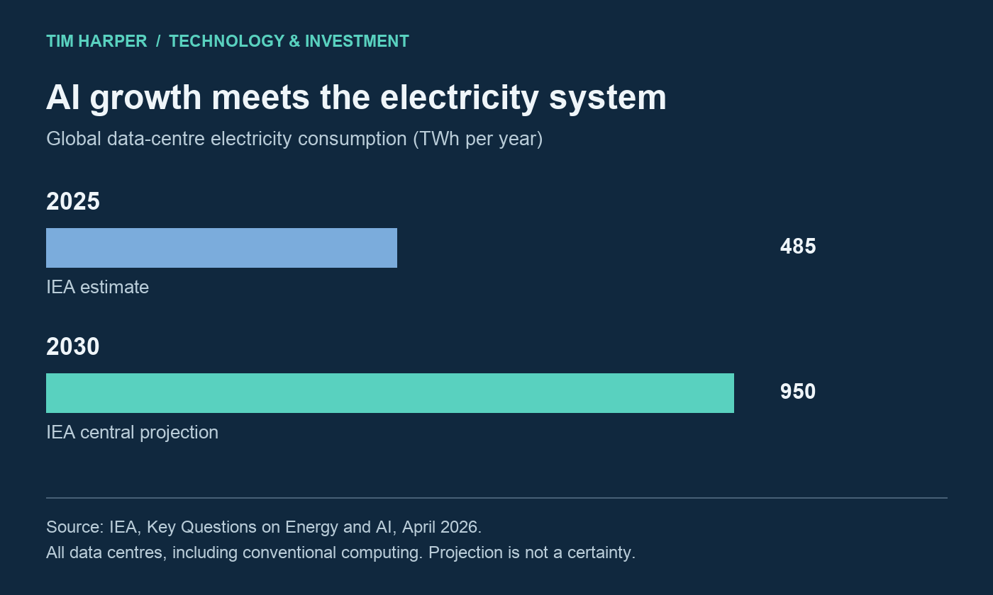
The scale makes that distinction consequential. The International Energy Agency reports that capital expenditure by five large technology companies exceeded $400 billion in 2025 and estimates a further 75% increase in 2026. That is company capital expenditure, not an audited total of spending exclusively on AI. Even with that qualification, the commitments are extraordinary. The IEA’s April 2026 assessment projects worldwide data-centre electricity consumption rising from 485 TWh in 2025 to 950 TWh in 2030. These figures cover all data centres, including conventional computing.
For an investor, impressive growth is only the beginning of the enquiry. A customer can gain substantially from a cheaper service while its supplier struggles to recover the cost of providing it. A useful model can attract millions of users without generating enough cash to replace the equipment on which it runs. At this scale, a business that looks primarily digital becomes increasingly exposed to the price and availability of physical capacity. The invoice for infrastructure arrives on a rather less speculative timetable than the productivity dividend.
Research checked 21 September 2026.
Two routes to an AI winter
An AI winter, in the investment sense used here, would be a sustained contraction in funding and deployment after expectations outrun commercial reality. It need not mean that researchers stop making progress or that customers stop using AI. Financial scarcity is the familiar route: revenues, margins and cash generation fail to justify the money committed, lenders become more demanding and new projects lose their funding.
There is another route. AI could succeed quickly enough to encounter shortages of the resources required to deliver it. Graphics processing units, or GPUs, perform much of the parallel arithmetic. They need high-bandwidth memory, or HBM: stacked memory placed close to the processor so that data can reach it quickly. Manufacturing the logic chip, producing the memory and joining them through advanced packaging are separate industrial tasks. More capacity in one does not automatically remove a bottleneck in another.
Memory manufacturer Micron’s June 2026 earnings remarks describe tight supply and rising AI-driven demand. HBM also draws on the manufacturing resources used for dynamic random-access memory, or DRAM, the working memory used more widely in computers. Beyond silicon sit cooling systems, electrical distribution equipment, transformers, generation and transmission. A completed server building cannot negotiate with an unfinished substation.
Physical scarcity can cause financial scarcity. More expensive components, longer delivery times and idle equipment raise the cost of delivering useful computation, other things equal. An application must then earn more revenue, achieve better utilisation or become more efficient to clear the same investment hurdle. Falling cost per task can still offset those pressures; scarcity does not imply that every AI price rises. But a financing model built around uninterrupted cost reductions becomes more vulnerable.
The squeeze will also be uneven. A scarce component may produce excellent returns for its supplier while weakening those of the operator buying it. That operator may pass the cost to customers, absorb it or abandon marginal applications. New capacity could eventually reverse a shortage and lower prices, to the benefit of later customers rather than its original financiers. “AI investment” covers several businesses with different customers, replacement cycles and bargaining power. Treating them as one trade conceals much of the economics.
The cost of finding out what happened
Cheap and increasingly abundant computation has encouraged engineers to solve information problems by processing more data. Often that is sensible. General-purpose hardware and adaptable software can be cheaper to develop than a dedicated device. As processing, bandwidth and power become more economically significant, the relevant comparison is how cheaply and reliably a system can obtain the information needed for a useful decision. There can be an extraordinary asymmetry between the information consumed by a system and the commercially useful information it produces.
Amazon’s Just Walk Out technology provides a useful illustration. Amazon describes cameras, shelf weight sensors and machine learning working together to establish who took what. The input is a complex account of activity in a shop; the valuable output is a reliable allocation of products to customers. Its RFID offering for clothing uses radio-frequency identification tags read at the exit to support another shopping format. This is evidence of different sensing architectures, not proof that Amazon changed course because computation was too expensive.
Robotics makes the asymmetry easier to quantify. One 4K image at 3,840 by 2,160 resolution contains 8,294,400 pixels. At 30 frames a second, that becomes 248,832,000 pixel observations each second. An uncompressed, 24-bit RGB stream contains approximately 746 MB/s, or 5.97 Gbit/s, before downstream processing. These are decimal units and a raw-data calculation, not a claim that every robot transmits or analyses full-resolution video. Compression, cropping and local processing can reduce the burden substantially.
A machine may process that stream to discover something quite small: an object moved, contact changed, a gripped component is beginning to slip, or too much force is being applied. The physical world contains much more information than the immediate control decision needs. Reconstructing a rich description of it can be valuable, but it is not automatically the cheapest route to a dependable answer.
The question becomes: what is the cheapest way of knowing it? Sometimes inference from a camera will win because it performs several jobs with one sensor. Sometimes a force sensor or tactile surface can measure the relevant contact condition more directly. Radar may suit a particular distance measurement. An event camera reports changes in brightness asynchronously instead of repeatedly recording an entire frame. Its data advantage depends on the scene; rapid motion or flickering illumination can generate many events.
Direct sensing is not free either. Sensors need integration, calibration and maintenance; tactile surfaces wear; readings may still require inference. The correct comparison includes reliability, latency and the cost of mistakes. As explored in why better AI increases the importance of robot touch, perception and intelligence are complementary. Better sensing can make a model more useful while reducing the work required to reach a particular decision.
A useful analytical framework is the economic value of information divided by the cost of acquiring and processing it. This is a way of examining architecture, not an established accounting ratio. Its value is that it shifts attention from the amount of computation performed to the useful decision purchased. Better measurement can sometimes avoid processing more data, provided it answers the same question with sufficient reliability.
Efficiency becomes a form of infrastructure
Resource scarcity puts a price on avoiding unnecessary computation. Smaller models, sparse inference that activates only the parts needed for a task, and specialised silicon can become more valuable. An application-specific integrated circuit, or ASIC, trades some flexibility for hardware designed around particular work. Edge processing moves computation closer to the sensor or user, potentially avoiding transmission and central processing, although it can also duplicate hardware across many devices.
The investment case depends on the whole system. Development costs can make a specialised chip unattractive at low volumes. A smaller model that requires frequent human correction may save electricity and lose money. A sensor that eliminates computation but makes a production line less reliable is an expensive economy. Efficiency must preserve the useful outcome, including the acceptable error rate.
Where it does, the saving can extend beyond the electricity bill. Lower peak demand may avoid an accelerator purchase, release memory capacity, reduce cooling requirements or postpone an electrical upgrade. A megawatt that does not have to be consumed can become as economically valuable as a megawatt of additional capacity, particularly when that megawatt determines whether another productive workload can run.
The qualification matters. A reduction in processor activity does not proportionally shrink every transformer or recover sunk expenditure on a building. Some equipment must remain sized for peak demand and redundancy. Savings are greatest when they release the actual constraint or prevent a future investment. In that sense efficiency is virtual infrastructure: it creates room to do more with resources already available.
Nor does better efficiency guarantee lower aggregate electricity demand. Cheaper tasks can encourage greater use, and developers can spend the saving on more capable models. That rebound does not invalidate the saving per useful result. It means that the benefits may appear as additional output and higher capacity utilisation rather than a smaller national electricity bill. Where efficiency cannot release enough of the binding constraint, the availability of actual electrical capacity becomes decisive.
Power has a location, a delivery date and a price
Data-centre demand is geographically concentrated. A manageable addition to global electricity consumption can be a severe problem for a particular network. JLL’s February 2026 research puts average connection timelines for large new loads in major data-centre markets at approaching five years. Its 2026 outlook describes operators funding generation themselves as grid delays encourage “bring your own power” arrangements. CBRE’s latest North American survey likewise identifies transmission and energisation delays as development constraints.
A hypothetical £50/MWh supply available today is economically different from a £50/MWh supply that cannot be connected until 2032. Time, location and availability each have a price. CBRE Investment Management’s analysis of powered land describes the resulting scarcity premium for sites with credible electricity access. That premium needs site-level scrutiny: proximity to a power line is not a firm, transferable right to use its capacity.
There is a limit to what earlier power is worth. For an illustrative 30 MW load operating at 90% utilisation, a £100/MWh premium costs £23.65 million a year. That premium makes sense only if the contribution earned by opening earlier, after other incremental costs and risks, exceeds the extra bill. It cannot be justified merely by pointing to the total capital cost of the data centre.
Private wires connecting generation directly to a customer can help where geography permits. Batteries can shift energy and support reliability; flexible workloads can sometimes move in time or location. Each approach has an engineering boundary. A battery still needs charging, a private wire still needs consent and equipment, and a latency-sensitive service cannot necessarily follow cheap wind around the country. The existing analysis of AI data centres and UK grid capacity examines this deployment problem.
Meanwhile, electricity can have very little value on the wrong side of a network bottleneck. NESO, Britain’s National Energy System Operator, reported £2.7 billion of total balancing costs in financial year 2024/25, rather than the roughly £2 billion sometimes cited. Its 2025 annual report identified increased thermal constraints, where intended power flows exceed network capability, as a principal driver. Wind curtailment reached 13% of hypothetical wind output without curtailment. These are dated annual figures, not a September 2026 running total.
The same report modelled balancing costs peaking around £8 billion in 2030, with timely and accelerated network delivery potentially avoiding about £4 billion of that peak. That is a conditional projection, not an unavoidable bill. Total balancing costs also include services beyond wind curtailment. My 2026 wind-curtailment analysis separates those measures.
Negative prices require equal care. NESO’s balancing-market evidence explains that a negative wind bid can mean the generator is paid to reduce output, including compensation for lost support payments. It is not an offer to sell an electrolyser free electricity. A producer needs a physical connection, an electricity contract and enough operating hours. The economic opportunity lies in overcoming the constraint, not in misreading a minus sign.
Hydrogen can move energy, at a considerable cost
Hydrogen is one possible way of moving energy across this mismatch in place and time. Renewable electricity can split water in an electrolyser near abundant or low-value generation. The hydrogen can then be stored for later use or transported beyond an electricity-network constraint to a place where firm power has greater value. This adds equipment, handling and substantial losses. The economic question is whether storage, transport and availability justify those costs in a particular case.
Consider an illustrative electrolyser consuming 50 kWh per kilogram. Hydrogen contains about 33.3 kWh/kg on a lower-heating-value basis, which excludes recovery of heat from condensing the water produced. At an assumed 50% net electrical conversion efficiency, a kilogram delivers 16.65 kWh. The electricity-to-hydrogen-to-electricity round trip is therefore about 33% before additional compression, storage and transport losses. Using electricity directly is far more energy-efficient. Where adequate firm electricity is already available, converting it to hydrogen and back will usually be difficult to justify. But round-trip efficiency does not measure the value of moving energy to where and when it can be used. The loss is a cost of providing that service, not by itself a measure of its value.
The 50 kWh assumption is deliberately transparent. DOE’s PEM electrolysis table gives 55 kWh/kg as its 2022 system status and 51 kWh/kg as a 2026 target. Its 48 kWh figure is a stack target, excluding some system consumption. A 48–52 kWh/kg sensitivity range is useful for an efficient-system scenario, but should not be presented as verified performance across the installed fleet.
At 50 kWh/kg, the electricity component of hydrogen production is straightforward:
| Renewable electricity price | Electricity cost per kg of hydrogen |
|---|---|
| £10/MWh | £0.50 |
| £20/MWh | £1.00 |
| £30/MWh | £1.50 |
| £40/MWh | £2.00 |
| £50/MWh | £2.50 |
These are calculations, not delivered hydrogen prices. Electrolyser capital recovery, financing, water treatment, maintenance, compression, storage, distribution and margin must be added. An electrolyser running only during occasional curtailment periods spreads its fixed costs over very few kilograms. Dedicated renewable supply, sometimes complemented by other contracted electricity, can improve utilisation but changes the input price. The model belongs at the renewable production site, not automatically on the constrained grid serving the data centre.
At the assumed conversion efficiency, every £1/kg in delivered hydrogen cost contributes roughly £60/MWh to the fuel cost of electricity. Thus £5/kg means about £300/MWh before paying for the generating plant, maintenance and reserve capacity. That is expensive against ordinary wholesale electricity, but a wholesale price is a poor comparator if the electricity cannot be delivered to the site. Cheap renewable input is several commercial steps away from cheap, reliable electricity at the destination.
Consider a hypothetical data centre that needs power in 2028 but cannot obtain adequate grid capacity until 2032. The comparison is between systems capable of covering that four-year gap, not between hydrogen and a cheaper grid supply that is unavailable. Hydrogen would have to justify its total cost against the value of earlier operation, including the contribution from compute that would otherwise be delayed, and against other deliverable solutions. Its conversion losses increase the price difference needed to make the case; they do not settle the comparison on their own. As with computation, the useful output matters more than the volume of input: here it is reliable power at the required place and time. Hydrogen remains only a candidate. Fuel availability, daily tonnage, storage, generation equipment, redundancy, permissions and logistics would all have to be demonstrated. A proposed hydrogen plant does not solve a current connection delay.
Natural-gas generation is a serious competitor where fuel access and emissions permissions allow it, though turbines and grid-independent reliability have their own constraints. Batteries, private-wire renewables, flexible demand and temporary or staged grid capacity may be preferable where they can meet the duty cycle. Grid reinforcement offers lasting value. Diesel retains limited backup roles, while nuclear, including potential small modular reactors, belongs in longer-horizon comparisons. Combinations may work better than any single option. Microsoft’s three-megawatt hydrogen fuel-cell demonstration established a backup-power use case, not the commercial competitiveness of continuous hydrogen generation. Renewable provenance and full supply-chain emissions must also be checked.
A large customer changes the hydrogen calculation
AI infrastructure and low-emissions hydrogen have almost inverse problems. One has rapidly growing demand straining its physical supply; the other has a substantial proposed supply pipeline without enough bankable customers. The IEA’s Global Hydrogen Review 2026 records almost 1 million tonnes of low-emissions production in 2025 and installed water-electrolysis capacity exceeding 4 GW. Only about 20% of newly signed offtake volumes in 2025 carried firm contractual commitments. Low-emissions hydrogen includes routes other than renewable electrolysis; it is not synonymous with green hydrogen.
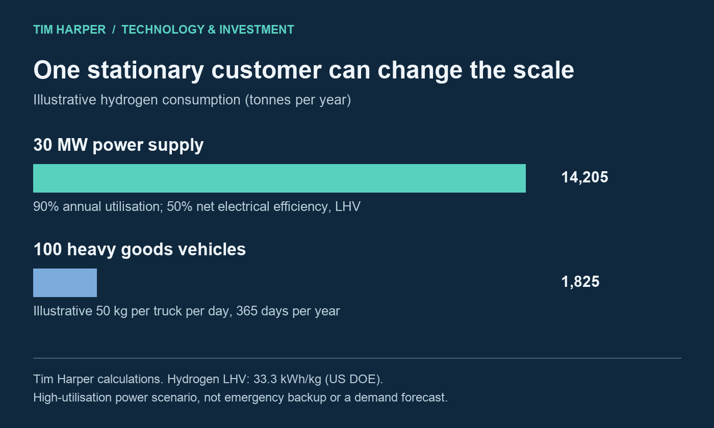
Scale makes stationary power interesting. A 30 MW electricity supply operating at 90% annual utilisation produces 236,520 MWh. At 50% electrical efficiency and 33.3 kWh/kg, it consumes approximately 14,205 tonnes of hydrogen a year. By comparison, 100 hydrogen heavy goods vehicles consuming an illustrative 50 kg each day throughout the year use 1,825 tonnes. The stationary application therefore matches roughly 778 such trucks. Actual vehicle consumption and operating days vary substantially.
This is a high-utilisation bridging-power scenario, not ordinary emergency backup. Producing its hydrogen at 50 kWh/kg requires approximately 710 GWh of electricity annually before downstream logistics, equivalent to an average electrolyser load of 81 MW. Intermittent renewables require greater installed capacity and suitable storage. Average hydrogen demand approaches 39 tonnes daily, so the delivery chain deserves as much attention as the generator.
A creditworthy customer signing a sufficiently durable contract could support larger renewable and electrolyser projects, improve financing terms and underpin storage and denser logistics. Transport and industrial customers could then provide incremental demand around infrastructure anchored by a larger buyer. The mechanism is shared infrastructure and better utilisation, not a data centre subsidising trucks. It addresses the coordination problem described in UK hydrogen infrastructure.
More demand alone does not make hydrogen cheaper; initially it could raise prices. Lower costs must come from scale, manufacturing volume, learning, financing or better utilisation of equipment and logistics. There is also a mismatch to negotiate: a data centre may need a bridge for a few years, while its hydrogen supplier needs revenue over a much longer asset life. Redeployment, alternative customers or appropriate termination payments would have to carry that risk.
Useful infrastructure can still destroy investor capital
The telecom boom offers a warning about ownership, timing and price when demand calls forth physical infrastructure. Federal Reserve Bank of San Francisco research found capital spending by publicly traded telecom service companies rising from $47 billion in 1995 to $121 billion in 2000, then falling to $49 billion in 2002. That is the study’s defined company sample, not a universal measure of US telecom investment. The underlying research also discusses differences between investment datasets.
Richmond Fed research describes excessive long-haul fibre capacity and investment overshooting. The OECD’s contemporary assessment documents heavy investor losses alongside continuing growth in communications use. The OECD also reported that telecoms accounted for 56.4% of the value of worldwide corporate bond defaults in 2002. Investors could be right that internet traffic would grow and still be wrong about how much infrastructure to build, how quickly, at what price and with whose borrowed money. Useful capacity survived financial failure; later customers and owners could capture value that the original investors did not.
AI need not repeat that history. Accelerators can become economically obsolete much faster than buried fibre, and power infrastructure has different lives and alternative uses. Those differences make asset selection more important. A future surplus might cheapen compute, memory, data-centre space and semiconductor capacity without making every unwanted accelerator useful or every grid connection transferable. Demand growth alone cannot settle what each asset will earn.
The two winters nevertheless lead back to the same discipline. If demand continues booming, constrained inputs increase the value of efficient computation and deliverable energy. If revenues disappoint, capital scarcity increases the value of efficiency and careful investment. If bottlenecks raise costs enough, the physical constraint can help trigger the financial correction. And if the response eventually builds too much capacity, later users may benefit while those who financed it absorb losses. Neither outcome is inevitable.
At scale, AI’s economics depend not only on the performance of its models but on the availability and cost of chips, memory, electricity and network capacity. That creates opportunities both in supplying more of those resources and in using less of them to produce the same useful result. Technological success does not guarantee a return to those who finance it.
References and calculation basis
Sources were checked on 21 September 2026. Forecasts remain the cited institutions’ estimates. The camera data rates, power premium and hydrogen comparisons are the author’s calculations from explicitly stated assumptions.
- The IEA’s April 2026 assessment
- June 2026 earnings remarks
- Amazon describes
- Its RFID offering for clothing
- event camera
- JLL’s February 2026 research
- 2026 outlook
- CBRE’s latest North American survey
- CBRE Investment Management’s analysis of powered land
- Private wires connecting generation directly to a customer
- 2025 annual report
- NESO’s balancing-market evidence
- 33.3 kWh/kg on a lower-heating-value basis
- DOE’s PEM electrolysis table
- Microsoft’s three-megawatt hydrogen fuel-cell demonstration
- IEA’s Global Hydrogen Review 2026
- The underlying research
- Richmond Fed research
- OECD’s contemporary assessment
- OECD also reported